Text Classification, Prediction and Bias Extraction using NLP

Text Classification for Hate Speech

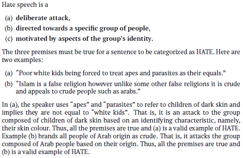
Our goal here is to build a Naive Bayes Model and Logistic Regression model on a real-world hate speech classification dataset. The dataset is collected from Twitter online. Each example is labeled as 1 (hatespeech) or 0 (Non-hatespeech).

Naive Bayes

Naive Bayes model was implemented with add-1 smoothing.

Trends observed

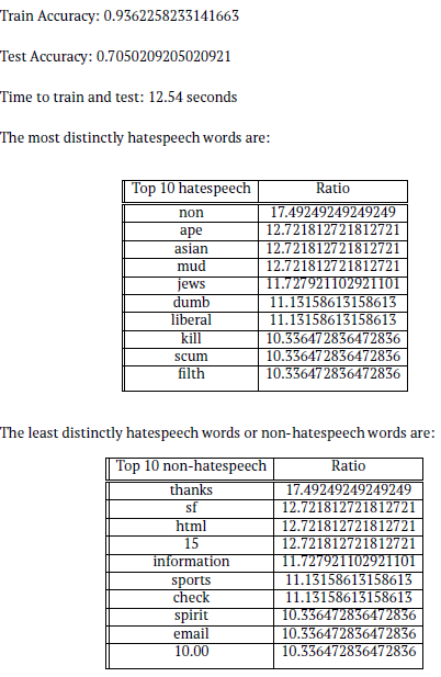
From the two tables above, it can be observed that the top 10 distinctly hatespeech words are words that are commonly used to describe people in a negative way. Some of these words are also directed at a person belonging to a specific race (e.g. asian), religion (e.g. jews), or a having certain political/moral leaning (e.g. liberal). The classifier is able to identify many hateful words correctly. On the other hand, the top 10 non-hatespeech words that were observed are random words like ”thanks”, ”information”, ”check”, or numbers like ”10.00” and ”15” which may not have much meaning in the context of a sentence.

Logistic Regression model

Accuracy results for LR model using unigram features:

Train Accuracy: 0.9804 Test Accuracy: 0.7285

From the above data,we can observe that both the models gave almost similar performance, however logistic regression model performed slightly better with train and test data. This slightly better performance of logistic regression could be attributed to logistic regression being better at generalization, as it does not assume independence between words like Naive Bayes does.

Comparison of both models with Perceptron classifier

• Naive Bayes and Logistic Regression models use separate training and test data. Perceptron classifier however, uses training data also as test data as this model learns online.
• The Perceptron classifier reads one sample instance at a time to learn about the data and update its understanding about it e.g If a prediction is incorrect, increases weights for features of the true label, and decreasesweights for features of the predicted label. On the other hand, Naive Bayes and Logistic Regression models read the entire sample dataset before updating their knowledge of the data.
• Observations about \lambda values varying from [0.0001, 0.001, 0.01, 0.1, 1, 10]

Observations:

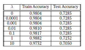
From the observations of accuracy with the different \lambda values, we can see that the test accuracy remains exactly the same for \lambda values of 0, 0.0001, 0.001, 0.01 and 0.1 and starts dropping at \lambda value 1 and furthermore at value 10. On the other hand, train accuracy remains same for 0, 0.0001 and 0.001. It shows a sight increase for each \lambda value from 0.001 to 0.1 to 1, and drops again at value 10. For \lambda = 1, train accuracy increases, but test accuracy drops. This may be due to over-fitting of data. As the train accuracy increases and test accuracy remain steady till 0.1, it can be concluded that \lambda = 0:1 value shows the highest accuracy.

Text Prediction with Language Modeling

This task involved implementing character level and word level n-gram language models along with a character level RNN language model.

Character level n-gram language model

Part 1: Generation

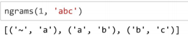
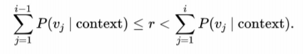
The function ngrams(n, text) produces a list of all ngrams of the specified size from the input text. Each ngram consists of a two element tuple (context, char), where the context is itself an n-length string comprised of the n characters preceding the current character. The sentence is padded with n~ characters at the beginning. If n = 0, all context is empty strings. We assume that n >= 0.

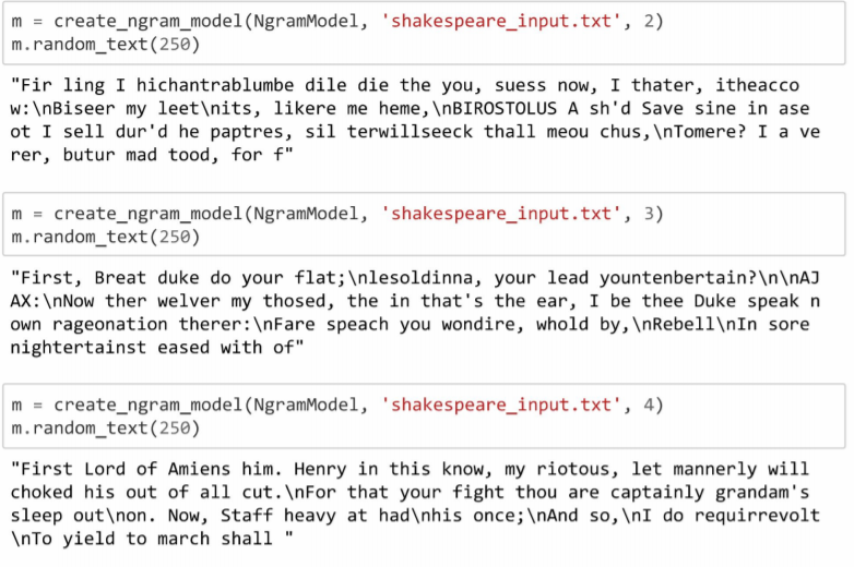
The function create_ngram_model(model_class, path, n, k) creates and returns an ngram model trained on the entire input file. The n-gram model, implemented using Python standard libraries, generates random text resembling the source document.

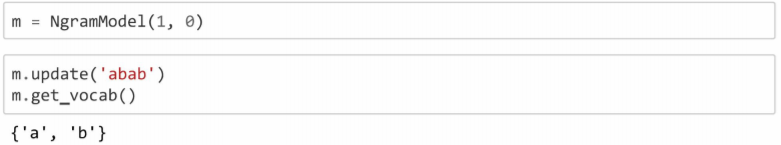
• The NgramModel class constructor initializes any necessary internal variables. The function get_vocab returns the vocabulary i.e set of all characters used by the model.

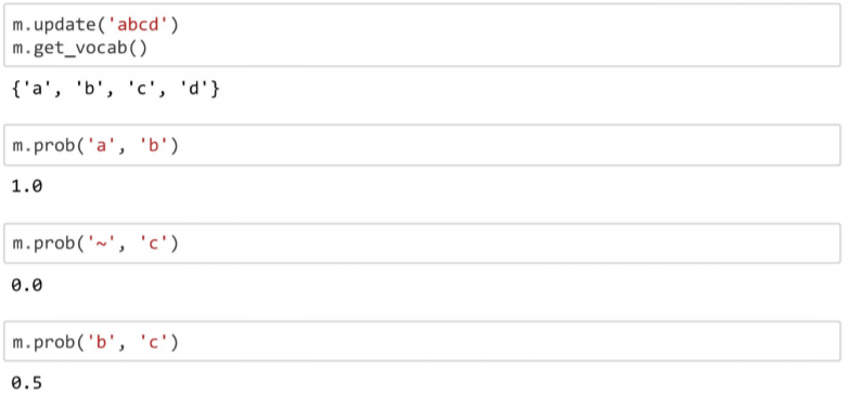
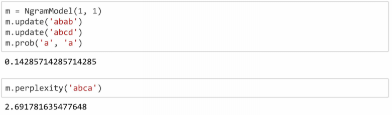
• The update(text) function computes the n-grams for the input sentences and updates the internal counts. the function prob(context, char) returns the probability of that character, given the preceding context. If a novel context is encountered the probability of any given char is set to 1/V where V is the size of the vocabulary.

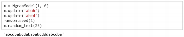
• The random_char(text) function returns a random character according to the probability distribution determined by the given context.

• The random_text function returns a string of characters chosen at random using random_char.

• Training the NgramModel with Shakespeare: The implemented language model is trained on a corpus of Shakespeare. The model generates sentences from Shakespeare with different order n-gram models.

Part 2: Perplexity, Smoothing and InterpolationL

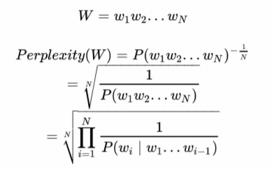
• Perplexity: To determine whether the language model is good, parlexity, the most common method for intrinsic metric of language models was implemented. The perplexity of alanguage model on a test set is the inverse probability of the test set, normalized by the number of characters.

• Smoothing: Laplace smoothing adds one to each count. Since there are V characters in the vocabulary and each one was incremented, the denominator is adjusted to take into account the extra V observations.

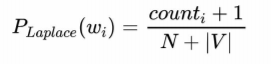
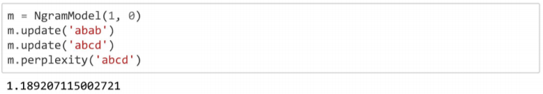
A variant of Laplace smoothing was implemented which adds k to each count instead of one.

• Interpolation: Interpolation helps avoid the problem of zeros if the longer sequence is not observed in our training data.

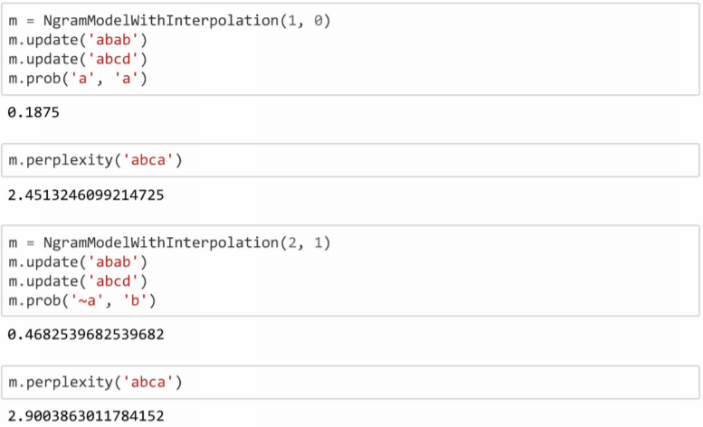
The class NgramWithInterpolation extenda NgramModel to implement interpolation. Add-k smoothing takes place only when calculating individual order n-gram probabilities.

Part 3: Observations:

Observations for the ngram language models where n ≥ 1,

• The paragraphs which character level models generate, all start with the letter ’F’.
• The paragraphs which word level models generate, all start with the word ’In’.

This is because, for character level models, as ’F’ is the starting letter of the input file, it is always chosen as the letter which has the highest probability of preceding other characters. As the value of n increases, the model repeated outputs ’First’ at the beginning of the paragraph. This is because, only characters that have a high probability of following the letter ’F’ are chosen as the next character. The word level model also works similarly. As ’In’ is the first word in the input file, it has the highest probability of preceding other words, which is why it is chosen repeatedly as the first word. When n = 0, all letters and words are independent of context, hence any character of letter can be chosen as the first one.

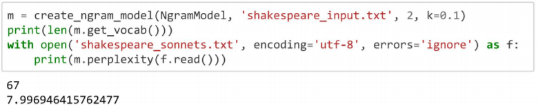
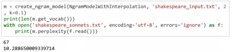
Perplexity of Shakespeare corpus for: (i) Character-level n-gram model: 10.2887 (ii) Word-level n-gram model: 6095.0115

From the perplexities observed for both the models, we can see that the character-leveln-gram model has a much lower perplexity than that of the word-level model. It is evident that character level n-gram model performs better than the word leveln-gram model.However, on observing the generated text, especially those for higher order languagemodels wheren≥3, the word-level n-gram model shows a much better result. Thesentences generated by the word level model seem much more coherent than thoseof the character level n-gram model. From the sample text generated by both modelsshown below, it can be observed that the sentences generated by the word-levelmodel make more sense than he character level model.Sample text generated by character-level n-gram model(n= 4): ”First Lord of Amiens him. Henry in this know, my riotous, let mannerly will chokedhis out of all cut.For that your fight thou are captainly grandam’s sleep out on. Now,Staff heavy at had his once; And so, I do requirrevolt To yield to march shall” Sample text generated by word-level n-gram model(n= 4).

”In the immediate term , though , that the negotiations with his own cabinet hadbeen rather less successful , as he has purportedly said in his letters . [E0S] They wereeventually allowed to travel outside the country and escaped . [E0S] Neverthelessthe new form brought new questions - “ How do you create the spontaneity andchemistry in a medium that ’s still evolving . [E0S] New fans : Lots of viewersexpressed their respect for George ’s attitude to life after last night ’s draw as Lottotickets sold at more than 200 a second in the hour before ticket sales close at 19:30GMT ahead of the draw at 20:30 on Wednesday”

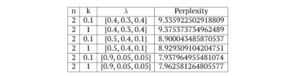
• Character-level n-gram model: Observations with n,k and λ. The best performance was observed with n= 2, k = 0.1 and [0.9,0.05,0.05], which gives a perplexity of 7.937964955481074.

• Word-level n-gram model: Observations with n,k and λ

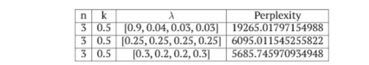
The best performance was observed with n= 3, k= 0.5 and [0.3,0.2,0.2,0.3], which gives a perplexity of 5685.745970934948 Word-level n-gram model: Observations with n, k and λ.

Exploring Bias from word analogies:

The pretrained word2vec embeddings are loaded from the GenSim package:

import gensim.downloader as api api.load(“word2vec-google-news-300”)

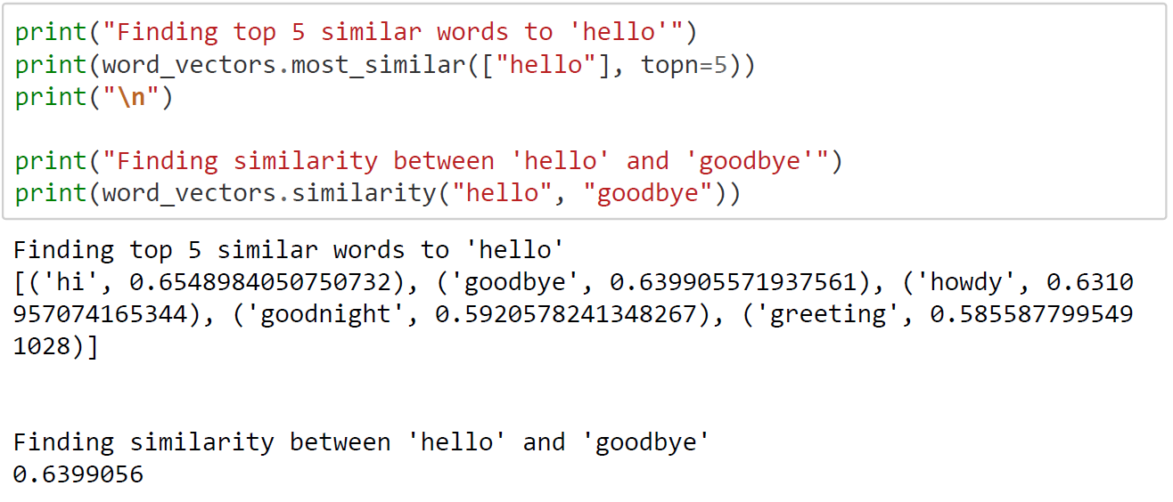
The loaded word_vectors in memory can be accessed like a dictionary to obtain the embedding of any word. GenSim provides a simple way out of the box to find the most similar words to a given word.

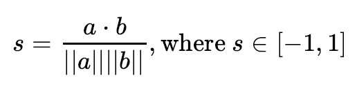
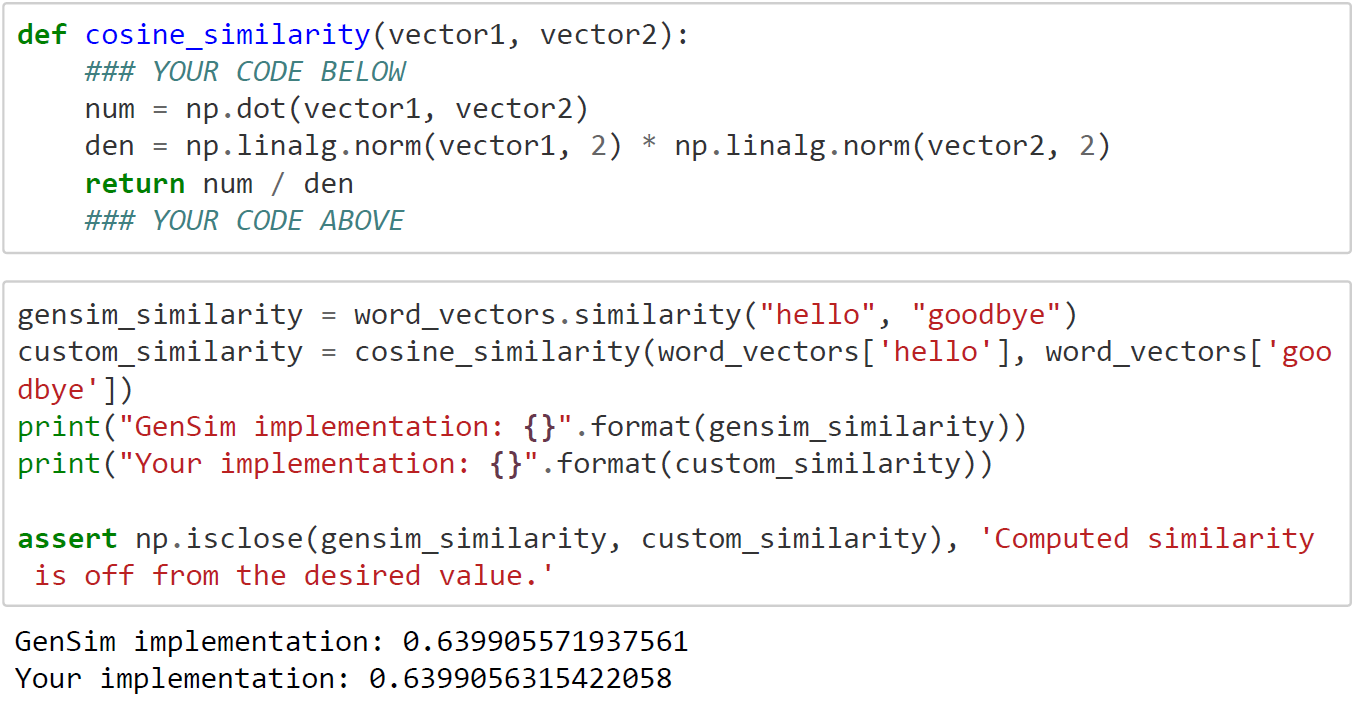
• Cosine Similarity: For quantifying simiarity between words based on their respective word vectors, a common metric is cosine similarity. Formally the cosine similarity between two vectors and, is defined as:

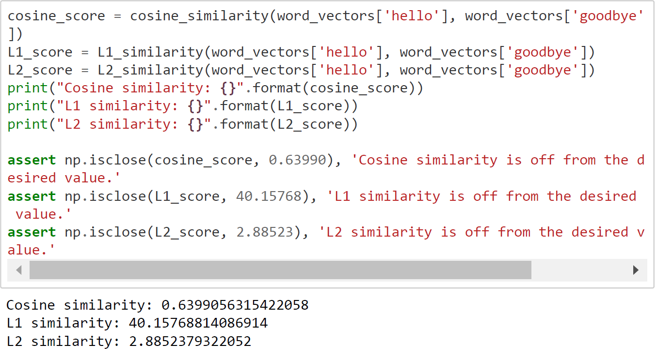
• L1 and L2 Similarity:

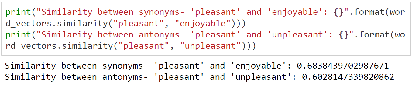
• Synonyms and Antonyms: In general, you would expect to have a high similarity between synonyms and a low similarity score between antonyms. For e.g. “pleasant” would have a higher similarity score to “enjoyable” as compared to “unpleasant”. However, counter-intuitievely this is not always the case. Often, the similarity score between a word and its antonym is higher than the similarity score with its synonym. For e.g. “sharp” has a giher similarity score with “blunt” as compared to “pointed”.

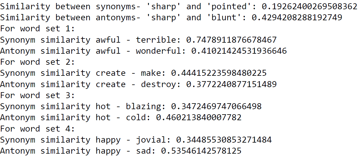
As it can be seen from the last two examples above, the words ‘hot’ and ‘happy’ have a higher similarity ratio with their respective antonyms than their antonyms. The reason for this is that word2vec does not capture similarity based on context rather than synonymy. e.g. In the sentence “The weather was —–”, in this context the missing word is more likely to be either ‘hot’ or ‘cold’, rather than blazing. Hence, the similarity between ‘hot’ and ‘cold’ is higher than that between ‘hot’ and ‘blazing’. Similarly, the words ‘happy’ and ‘sad’ are more likely to occur in the same context than ‘happy’ and jovial’.

• Analogies: The Distributional Hypothesis which says that words that occur in the same contexts tend to have similar meanings, leads to an interesting property which allows us to find word analogies like “king” - “man” + “woman” = “queen”.

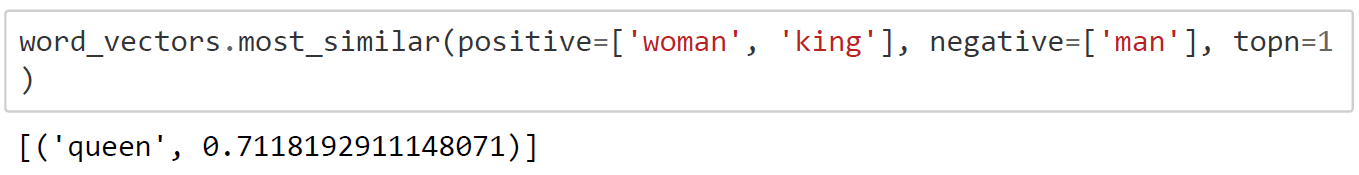
The analogy man:king::woman:queen holds true even when looking at the word embeddings.

• Bias: Often, bias creeps into word embeddings. This may be gender, racial or ethnic bias. Let us look at an exampleman: doctor::woman:? gives high scores for “nurse” and “gynecologist”, revealing the underlying gender stereotypes within these job roles.

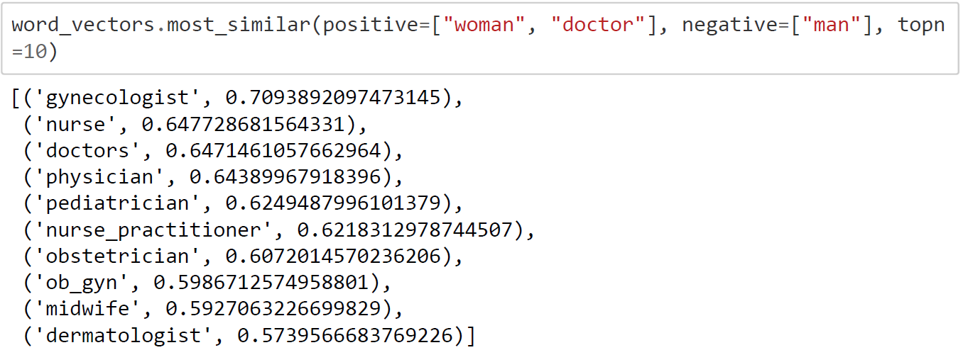
The examples observed above are stereotypical gender biases which are widely observed in languages. The reason for the existence of this bias can be traced to the text data the word2vec model is trained on. These text data reflect the common human biases related to gender, race, religion etc. The more that models are trained on these text data, the more these biases are amplified.